Statistics 1. Summarizing Quantitative data

Originally published in Kaggle

Introduction

Quantitative data is information that can be measured in real numbers. Examples include,

Height of a person
Speed of Tesla cars
Runs scored by a batsman
Wickets taken by a bowler

In this notebook, we'll explore various statistical concepts involved in summarizing quantitative data with the help of Indian Premier League (IPL) dataset.

The data consists of two CSV files for all IPL matches played from 2008 - 2018 (11 seasons)

matches.csv - match-by-match data
deliveries.csv - ball-by-ball data

Let's setup pandas dataframes for the above files and import necessary libraries.

import math
import numpy as np
import pandas as pd
from scipy import stats
import os

matches    = pd.read_csv('../input/matches.csv')
deliveries = pd.read_csv('../input/deliveries.csv')

Let's inspect the matches data before stepping into the concepts

print(f'Number of rows    = {len(matches)}')
print(f'Number of columns = {len(matches.columns)}')
matches.head()

Number of rows    = 696
Number of columns = 18

	id	season	city	date	team1	team2	toss_winner	toss_decision	result	winner	win_by_runs	win_by_wickets	player_of_match	venue	umpire1	umpire2	umpire3
0	1	2017	Hyderabad	2017-04-05	Sunrisers Hyderabad	Royal Challengers Bangalore	Royal Challengers Bangalore	field	normal	Sunrisers Hyderabad	35	0	Yuvraj Singh	Rajiv Gandhi International Stadium, Uppal	AY Dandekar	NJ Llong	NaN
1	2	2017	Pune	2017-04-06	Mumbai Indians	Rising Pune Supergiant	Rising Pune Supergiant	field	normal	Rising Pune Supergiant	0	7	SPD Smith	Maharashtra Cricket Association Stadium	A Nand Kishore	S Ravi	NaN
2	3	2017	Rajkot	2017-04-07	Gujarat Lions	Kolkata Knight Riders	Kolkata Knight Riders	field	normal	Kolkata Knight Riders	0	10	CA Lynn	Saurashtra Cricket Association Stadium	Nitin Menon	CK Nandan	NaN
3	4	2017	Indore	2017-04-08	Rising Pune Supergiant	Kings XI Punjab	Kings XI Punjab	field	normal	Kings XI Punjab	0	6	GJ Maxwell	Holkar Cricket Stadium	AK Chaudhary	C Shamshuddin	NaN
4	5	2017	Bangalore	2017-04-08	Royal Challengers Bangalore	Delhi Daredevils	Royal Challengers Bangalore	bat	normal	Royal Challengers Bangalore	15	0	KM Jadhav	M Chinnaswamy Stadium	NaN	NaN	NaN

Measuring center

First step often learnt in descriptive statistics is to measure the center of given data. There are various ways to measure the center. We'll go through some of them.

Let's get the data ready for our experiments.

win_by_runs columns represents the margin in which a team has won against the opponent, if the team batting first has won.
i.e. If team1 scores 200 runs and team2 scores 150 runs, team1 won the match by 50 runs - If team1 bats first

Hence, we have to exclude all instances of win_by_wickets cases, i.e. win_by_runs = 0

win_by_runs_data = matches[matches['win_by_runs'] > 0].win_by_runs
print(f'Number of rows = {len(win_by_runs_data)}')
win_by_runs_data.head()

Number of rows = 315





0     35
4     15
8     97
13    17
14    51
Name: win_by_runs, dtype: int64

We'll discuss about 3 methods of measuring center - Mean, Median and Mode

Mean

Mean (usuallly refered to Arithmetic Mean, also called Average) is calculated as sum of all numbers in the dataset and dividing by the total number of values

Arithmetic Mean

Arithmetic\,mean = {Sum\,of\,all\,numbers \over No.\,of\,values\,in\,the \,set}\,\,\,\,or\,

\bar{x} = {\sum_{i=i}^{n} x_{i} \over n}

Arithmetic mean of our data is calculated as,

mean = (35 + 15 + 97 + 17 + ...) / 315

Let's do that in code.

win_by_runs_rows = len(win_by_runs_data) # No. of values in the set (n)
win_by_runs_sum = sum(win_by_runs_data) # Sum of all numbers

print(f'Sum of all numbers = {win_by_runs_sum}, No. of values in the set = {win_by_runs_rows}')

win_by_runs_arithmetic_mean = win_by_runs_sum / win_by_runs_rows # Calculating arithmetic mean
print(f'Arithmetic mean = {win_by_runs_arithmetic_mean}')

Sum of all numbers = 9377, No. of values in the set = 315
Arithmetic mean = 29.76825396825397

We can verify the number with the help of mean() method in pandas

win_by_runs_arithmetic_mean_verify = win_by_runs_data.mean()
print(f'Arithmetic mean (verify) = {win_by_runs_arithmetic_mean_verify}')

Arithmetic mean (verify) = 29.76825396825397

Geometric Mean

Another type of mean is geometric mean. It is calculated as Nth root of product of all the numbers, where N is the total number of values in the dataset

Geometric\,mean = \sqrt[n]{product\,of\,all\,numbers}

\bar{x}_{geom} = \sqrt[n]{\prod_{i=1}^n x_i}

Geometric mean of our data is calculated as,

geometric_mean = 315thRoot(35 x 15 x 97 x 17 x ...)

win_by_runs_geo_mean = stats.mstats.gmean(win_by_runs_data)
print(f'Geometric mean = {win_by_runs_geo_mean}')

Geometric mean = 19.272304223934352

Median

Median is the middle value, when the data is sorted in ascending order. Half of the data points are smaller and half of data points are larger than the median.

For example purpose, let's take first 10 entries of the data.

win_by_runs_10 = list(win_by_runs_data[:10])
print(win_by_runs_10)
print(sorted(win_by_runs_10))

[35, 15, 97, 17, 51, 27, 5, 21, 15, 14]
[5, 14, 15, 15, 17, 21, 27, 35, 51, 97]

To find median,

Sort the data from smallest to largest (ascending order)
If there are odd number of data points, median is the middle data point.
If there are even number of data points, median is the average of two middle data points

[5, 14, 15, 15, 17, 21, 27, 35, 51, 97]
                ^^  ^^  
           (middle numbers)
                                  
Median = (17 + 21)/2 = 19

Let's verify,

win_by_runs_10_median = win_by_runs_data[:10].median()
print(f'Median (first 10) = {win_by_runs_10_median}')

win_by_runs_median = win_by_runs_data.median()
print(f'Median = {win_by_runs_median}')

Median (first 10) = 19.0
Median = 22.0

Mode

Mode is the number occurring most often in the dataset.

It is only meaningful if we have many repeated values in our dataset
If no value is repeated, there is no mode
A dataset can have one mode, multiple modes or no mode.

Let's try to retrieve mode for our dataset.

# Retrieve frequency (sorted, descending order)
win_by_runs_data.value_counts(sort=True, ascending=False).head()

4     11
14    11
10    10
15     9
13     9
Name: win_by_runs, dtype: int64

As we can observe, [4, 14] occurs 11 times in the dataset.

Hence, Mode = [4, 14],

We can verify using pandas.DataFrame.mode method

win_by_runs_data_mode = win_by_runs_data.mode()
print(f'Mode = {list(win_by_runs_data_mode)}')

Mode = [4, 14]

Measuring spread (variability)

By just measuring the center of the data, one wouldn't get much idea about the dataset. There are various ways of measuring how the data is spread.

Range

Range is the simplest form of measuring variability. It is the difference between largest number and smallest number.

win_by_runs_max = win_by_runs_data.max()
win_by_runs_min = win_by_runs_data.min()
win_by_runs_range = win_by_runs_max - win_by_runs_min

print(f'Largest = {win_by_runs_max}, Smallest = {win_by_runs_min}, Range = {win_by_runs_range}')

Largest = 146, Smallest = 1, Range = 145

Interquartile Range (IQR)

Interquartile range or IQR is the amount spread in middle 50% of the dataset or the distance between first Quartile (Q₁) and third Quartile (Q₃)

First Quartile (Q₁) = Median of data points to left of the median in ordered list (25th percentile)
Second Quartile (Q₂) = Median of data (50th percentile)
Third Quartile (Q₃) = Median of data points to right of the median in ordered list (75th percentile)
IQR = Q₃ - Q₁

Interquartile range

[41, 48, 58, 60, 60, 67, 69, 71, 75, 78, 81, 83, 89, 89, 91, 92, 94, 94, 96, 98]
 ^^^^^^^^^^^^^^^^^^^^^^^^^^^^^^^^^^^^^^  ^^^^^^^^^^^^^^^^^^^^^^^^^^^^^^^^^^^^^^
             first half                              second half
        median = (60 + 67) / 2 = 63.5        median = (91 + 92) / 2 = 91.5

Q₁ = 63.5
Q₃ = 91.5
IQR = Q₃ - Q₁ = 91.5 - 63.5 = 28

Let's calculate IQR for win_by_runs

win_by_runs_25_perc = stats.scoreatpercentile(win_by_runs_data, 25)
win_by_runs_75_perc = stats.scoreatpercentile(win_by_runs_data, 75)

win_by_runs_iqr = stats.iqr(win_by_runs_data)
print(f'Q1 (25th percentile) = {win_by_runs_25_perc}')
print(f'Q3 (75th percentile) = {win_by_runs_75_perc}')
print(f'IQR = Q3 - Q1 = {win_by_runs_75_perc} - {win_by_runs_25_perc} = {win_by_runs_iqr}')

Q1 (25th percentile) = 11.0
Q3 (75th percentile) = 38.0
IQR = Q3 - Q1 = 38.0 - 11.0 = 27.0


/opt/conda/lib/python3.6/site-packages/scipy/stats/stats.py:1713: FutureWarning: Using a non-tuple sequence for multidimensional indexing is deprecated; use `arr[tuple(seq)]` instead of `arr[seq]`. In the future this will be interpreted as an array index, `arr[np.array(seq)]`, which will result either in an error or a different result.
  return np.add.reduce(sorted[indexer] * weights, axis=axis) / sumval

Percentiles

Percentile is a number where certain percentage of numbers fall below that number.

Taking the above example,

25th percentile = 11 → 25% of the matches are won by less thant 11 runs.
75th percentile = 38 → 75% of the matches are won by less than 38 runs.

Percentile can be calculated using scipy.stats.scoreatpercentile

To calculate 95th percentile,

win_by_runs_95_perc = stats.scoreatpercentile(win_by_runs_data, 95)
print(f'95th percentile = {win_by_runs_95_perc}')

95th percentile = 86.0


/opt/conda/lib/python3.6/site-packages/scipy/stats/stats.py:1713: FutureWarning: Using a non-tuple sequence for multidimensional indexing is deprecated; use `arr[tuple(seq)]` instead of `arr[seq]`. In the future this will be interpreted as an array index, `arr[np.array(seq)]`, which will result either in an error or a different result.
  return np.add.reduce(sorted[indexer] * weights, axis=axis) / sumval

Variance and Standard deviation

Standard deviation and variance measures the spread of a dataset. If the data is spread out largely, standard deviation (and variance) is greater.

In other terms,

if more data points are closer to the mean, standard deviation is less
if the data points are further from the mean, standard deviation is more

Formula for variance for population is given as,

Variance\,=\sigma^2 = {\sum_{i=i}^{n}{(x_i - \mu)}^2 \over n}

where, $\mu$ is the mean of the dataset

Standard deviation is just the square root of variance

Standard\,deviation\,=\sigma = \sqrt{\sum_{i=i}^{n}{(x_i - \mu)}^2 \over n}

Note:

For Sample, we use n - 1 instead of n, $\bar{x}$ - mean of sample

Standard\,deviation\,=S_{sample} = \sqrt{\sum_{i=i}^{n}{(x_i - \bar{x})}^2 \over n - > 1}

Let's take win_by_wickets dataset.

win_by_wickets_data = matches[matches.win_by_wickets > 0].win_by_wickets
print(f'Number of rows = {len(win_by_wickets_data)}')
win_by_wickets_data.head()

Number of rows = 371





1     7
2    10
3     6
5     9
6     4
Name: win_by_wickets, dtype: int64

Let's calculate the standard deviation by formula

# Step 1: calculate mean(μ)
win_by_wickets_mean = win_by_wickets_data.mean()
print(f'Mean = {win_by_wickets_mean}')

# Step 2: calculate numerator part - sum of (x - mean)
win_by_wickets_var_numerator = sum([(x - win_by_wickets_mean) ** 2 for x in win_by_wickets_data])

# Step 3: calculate variane
win_by_wickets_variance = win_by_wickets_var_numerator / len(win_by_wickets_data)
print(f'Variance = {win_by_wickets_variance}')

# Step 4: calculate standard deviation
win_by_wickets_standard_deviation = math.sqrt(win_by_wickets_variance)
print(f'Standard deviation = {win_by_wickets_standard_deviation}')

Mean = 6.283018867924528
Variance = 3.3673396734984533
Standard deviation = 1.835031245918841

Let's verify the result using pandas.DataFrame.std (Note: We're passing ddof = 0 for population)

win_by_wickets_standard_deviation_verify = win_by_wickets_data.std(ddof = 0)
print(f'Standard deviation = {win_by_wickets_standard_deviation_verify}')

Standard deviation = 1.835031245918841

i.e. matches are won by an average of 6.28 wickets with standard deviation of 1.83 (spread = 6.28 $\pm$ 1.83)

Comparison with IQR

IQR is calculated with respect to median, Standard deviation is calculated with respect to mean.

Let's compare those for win_by_runs data

win_by_runs_std = win_by_runs_data.std(ddof = 0)
print(f'| Mean               = {win_by_runs_arithmetic_mean} | Median  = {win_by_runs_median} |')
print(f'| Standard deviation = {win_by_runs_std} | IQR     = {win_by_runs_iqr} |')

| Mean               = 29.76825396825397 | Median  = 22.0 |
| Standard deviation = 27.28719000229254 | IQR     = 27.0 |

For this particular data, standard deviation and IQR are pretty close by, although it won't be the scenario always.

Distribution graph

Let's plot the frequency distribution graph for win_by_wickets data since we can have values from 1 - 10.

win_by_wickets_dist = win_by_wickets_data.value_counts(sort=False)
plt = win_by_wickets_dist.plot.bar(color='lightblue')
plt.axvline(x = win_by_wickets_mean - 1, color='blue', linewidth=2.0)
plt.axvline(x = win_by_wickets_mean - win_by_wickets_standard_deviation - 1, color='red', linewidth=2.0, linestyle='dashed')
plt.axvline(x = win_by_wickets_mean + win_by_wickets_standard_deviation - 1, color='red', linewidth=2.0, linestyle='dashed')

<matplotlib.lines.Line2D at 0x7fdd0be0e828>

png

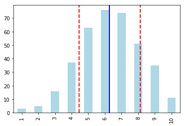
Blue line = Mean
Red line = Mean $\pm$ std.dev

Mean Absolute Deviation (MAD)

Mena absolute deviation is the average distance between mean and each data point.

Mean\,absolute\,deviation\,(MAD) = {\sum{\lvert x_i - \bar{x} \rvert} \over n}

Let's calculate mean absolute deviation for win_by_runs

win_by_runs_mad = win_by_runs_data.mad()
print(f'Mean absolute deviation = {win_by_runs_mad}')

Mean absolute deviation = 20.129644746787577

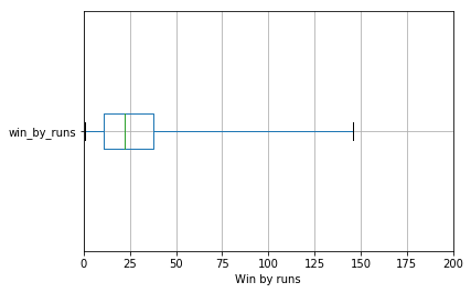
Box and whisker plots

Box and whisker plots (or box plots) represents five-number summary of the dataset. The five-number values are,

Minimum
First quartile (25th percentile)
Median (50th percentile)
Third quartile (75th percentile)
Maximum

The following is a representation of box-and-whisker plot

Box-whisker plot

plt = win_by_runs_data.to_frame().boxplot(whis='range', vert=False)
plt.set_xlim([0, 200])
plt.set_xlabel('Win by runs')

Text(0.5,0,'Win by runs')

png

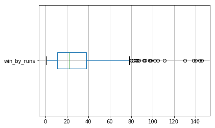
There's one problem with this graph. We have outliers to the right of the graphs. Instead of showing min and max as the two ends of the whisker, we calculate the following.

Lower fence = $Q_1 - 1.5 \times IQR$ ,
Upper fence = $Q_3 + 1.5 \times IQR$

Note the whis parameter in the above code set to range. By default whis is set to 1.5.

win_by_runs_data.to_frame().boxplot(vert=False)

<matplotlib.axes._subplots.AxesSubplot at 0x7fdd0babd320>

png