Descriptive Statistics

Categorical Data

A categorical variable (also called nominal variable) use labels or names with no numerical value.

Examples

• Continent (Asia, Africa, Europe, Australia, North America, South America, Antarctica)
• Color (Red, Green, Cyan, Blue)
• Laptop Brand (Apple, Lenovo, Microsoft, Dell)

Quantitative Data

Information that can be measured in numerical values which represent measurement, frequencies etc.

Examples

• No. of Users (50, 40, 67, 178, 207)
• Battery capacity in mAh (3100, 3200, 2800, 4000, 1500)
• Milk quantity in Litres (2.5, 1.35, 6.0, 5.4)

Frequency Distribution

Let's take a dummy dataset - 60 Users' car brands

| Audi | Audi | BMW | Audi | Porsche | Audi | | Ford | Audi | Volkswagen | BMW | BMW | Audi | | Porsche | Volkswagen | BMW | Audi | BMW | BMW | Audi | Porsche | Audi | Benz | BMW | Benz | | Volkswagen | BMW | Audi | Audi | Porsche | Porsche | | Audi | BMW | Audi | Audi | Porsche | Benz | | Benz | Porsche | Audi | BMW | Volkswagen | BMW | | Volkswagen | BMW | Audi | Audi | Porsche | Benz | Benz | Ford | Audi | Volkswagen | Benz | Ford | | Ford | Audi | BMW | Audi | Porsche | BMW |

import pandas as pd
import matplotlib

cars = ['Audi', 'Audi', 'BMW', 'Audi', 'Porsche', 'Audi', 
        'Ford', 'Audi', 'Volkswagen', 'BMW', 'BMW', 'Audi', 
        'Porsche', 'Volkswagen', 'BMW', 'Audi', 'BMW', 'BMW', 
        'Audi', 'Porsche', 'Audi', 'Benz', 'BMW', 'Benz', 
        'Volkswagen', 'BMW', 'Audi', 'Audi', 'Porsche', 'Porsche', 
        'Audi', 'BMW', 'Audi', 'Audi', 'Porsche', 'Benz', 
        'Benz', 'Porsche', 'Audi', 'BMW', 'Volkswagen', 'BMW', 
        'Volkswagen', 'BMW', 'Audi', 'Audi', 'Porsche', 'Benz', 
        'Benz', 'Ford', 'Audi', 'Volkswagen', 'Benz', 'Ford', 
        'Ford', 'Audi', 'BMW', 'Audi', 'Porsche', 'BMW'
]

cars_df = pd.DataFrame(cars, columns = ['brand'])
frequency_distribution = cars_df.brand.value_counts()
print(frequency_distribution)

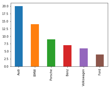
Audi          20
BMW           14
Porsche        9
Benz           7
Volkswagen     6
Ford           4
Name: brand, dtype: int64

Let's plot a Bar chart for the Frequency distribution

frequency_distribution.plot.bar()

Averaging data

Let's take an example data set of Marks of 20 students in a class out of 100.

import numpy as np
grades = [60, 75, 78, 48, 89, 94, 69, 98, 91, 71,
          89, 41, 67, 94, 60, 58, 96, 83, 81, 92]

Mean

Arithmetic Mean

Arithmetic mean is calculated as sum of all numbers in the dataset and dividing by the total number of values

Arithmetic mean = $\large{\mathsf{Sum\,of\,all\,numbers \over \#\,of\,values\,in\,the\,set}}$

= (60 + 75 + 78 + ... + 92) / 20 = 76.7

arithmetic_mean = np.mean(grades)
print(f'Arithmetic mean = {arithmetic_mean}')

Arithmetic mean = 76.7

Geometric Mean

Geometric mean is calculated as Nth root of Product of all the numbers, where N is the total number of values in the dataset

Geometric mean = $\mathsf{\sqrt[n]{Product\,of\,all\,numbers}}$

= $\sqrt[20]{60\times75\times78...\times92}$

from scipy.stats.mstats import gmean

geometric_mean = gmean(grades)
print(f'Geometric mean = {geometric_mean}')

Geometric mean = 74.69662039171091

Median

Median is the middle value, when the data is sorted in ascending order.

grades_sorted = sorted(grades)
print(grades_sorted)

[41, 48, 58, 60, 60, 67, 69, 71, 75, 78, 81, 83, 89, 89, 91, 92, 94, 94, 96, 98]
                                     ^^  ^^
                                    middle numbers
Hence, Median = (78 + 81) / 2 = 79.5

Let's verify,

grades_median = np.median(grades)
print(f'Median = {grades_median}')

Median = 79.5

Mode

Mode is the number occurring most often in the dataset

In our dataset, 89, 94 and 60 occurs two times.

Hence, Mode = 89, 94, 60

Measuring Variability of Data

Interquartile range (IQR)

Interquartile range or IQR is the amount spread in middle 50% of the dataset or the distance between first Quartile (Q₁) and third Quartile (Q₃)

• First Quartile (Q₁) = Median of data points to left of the median in ordered list
• Second Quartile (Q₂) = Median of data
• Third Quartile (Q₃) = Median of data points to right of the median in ordered list

[41, 48, 58, 60, 60, 67, 69, 71, 75, 78, 81, 83, 89, 89, 91, 92, 94, 94, 96, 98]
 ^^^^^^^^^^^^^^^^^^^^^^^^^^^^^^^^^^^^^^  ^^^^^^^^^^^^^^^^^^^^^^^^^^^^^^^^^^^^^^
             first half                              second half
        median = (60 + 67) / 2 = 63.5        median = (91 + 92) / 2 = 91.5

Q₁ = 63.5
Q₃ = 91.5
IQR = Q₃ - Q₁ = 91.5 - 63.5 = 28

Range

Range is the difference between largest number and smallest number

grades_range = max(grades) - min(grades)
print(f'Range = {grades_range}')

Range = 57

Variance

Variance measures how far the numbers are spread out from the mean.

• Variance, σ² = ${\sum (X - \mu)^2 \over n}$

print(f'Arithmetic mean = {arithmetic_mean}') # Mean

variance = ( sum([(x - arithmetic_mean) ** 2 for x in grades]) ) / 20
print(f'Variance = {variance}')

Arithmetic mean = 76.7
Variance = 5420.200000000001

Standard Deviation

Standard deviation is the square root of Varaince

• Standard Deviation, σ = $\sqrt{\sum (X - \mu)^2 \over n}$

std_deviation = np.sqrt(variance)
print(f'Standard Deviation = {std_deviation}')

Standard Deviation = 16.462381358722073

Z-Score

Z-Score is a measure of how many Standard Deviations above/below the Arithmetic mean a raw score is.

• Z-Score = ${X - \bar{x} \over \sigma}$

def z_score(raw_score, mean, std_deviation):
    """Calculates the statistical `z-score` value given `raw_score`, `mean`,
    and `std_deviation`

    Arguments:

    raw_score - Raw score
    mean - Mean
    std_deviation - Standard deviation
    """
    return (raw_score - mean) / std_deviation

z_score_60 = z_score(60, arithmetic_mean, std_deviation)
print(f'Z-score of 60 = {z_score_60}')

Z-score of 60 = -1.0144340381929031