Random Variables

A random variable is an unknown, whose possible values are numerical outcomes of a random phenomenon.

Example 1: Tossing a coin - we get Heads or Tails. If we associate values to each outcome, i.e. Heads = 0, Tails = 1, we can say,

$X = \{0, 1\}$

$X \color{red}{\leftarrow Random\,Variable},\,\,\{0,1\} \color{red}{\leftarrow Possible\,values}$

Example 2: Rolling a die - we get vaue between 1 and 6.

$Y = \{1, 2, 3, 4, 5, 6\}$

Random variable is denoted by uppercase letter (X, Y, ...)
Specific values are denoted by lowercase letters (x=0, y=5 etc.)

There are two types of random variables - Discrete and Continuous variables.

Discrete Variables

Discrete variables take only specific values

Examples

Outcomes of rolling a die
No. of players in a team
No. of smartphones in Toronto.

Continuous Variables

Continuous variables can take infinite number of values within a range

Examples

Weight of children from age 6-13
Time taken to hit first goal in soccer
Economy rates of a bowler in cricket

Probability distribution

Let's construct probability distribution for a discrete random variable. Given a dummy dataset of 40 ratings for a movie on a scale of 1 - 5 - ratings

import numpy as np
import pandas as pd

ratings = [5, 4, 4, 5, 1, 4, 3, 3, 5, 5,
           1, 1, 3, 5, 5, 4, 3, 5, 1, 5,
           5, 2, 5, 4, 5, 5, 3, 1, 1, 1,
           5, 4, 4, 4, 3, 5, 2, 1, 2, 4]
ratings_df = pd.DataFrame(ratings, columns = ['ratings'])
print(ratings_df.ratings.value_counts())

5    14
4     9
1     8
3     6
2     3
Name: ratings, dtype: int64

Let's calculate the probability distribution for each of rating value.

Rating	Responses	Probability distribution
5	14	14/40 = 35%
4	9	9/40 = 22.5%
3	6	6/40 = 15%
2	3	3/40 = 7.5%
1	8	8/40 = 20%

We can verify the same using pandas

ratings_distribution = ratings_df.ratings.value_counts(normalize = True) * 100
print(ratings_distribution)

5    35.0
4    22.5
1    20.0
3    15.0
2     7.5
Name: ratings, dtype: float64

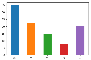
Let's plot the probability distribution graph.

import matplotlib

ratings_distribution.sort_index(ascending = False).plot.bar()

Probability Distribution - Ratings

Expected Value

Expected value is the weighted average of the possible values

For the above example, if X is the random variable,

X	P(X)	Weighted value
5	0.35	5 × 0.35 = 1.75
4	0.225	4 × 0.225 = 0.9
3	0.15	3 × 0.15 = 0.45
2	0.075	2 × 0.075 = 0.15
1	0.2	1 × 0.2 = 0.2

$ $Expected\,Value\,E(X) = 1.75 + 0.9 + 0.45 + 0.15 + 0.2 = 3.45 $$

We can verify by calculating the average,

ratings_avg = sum(ratings) / len(ratings)
print(f'Expected value = {ratings_avg}')

Expected value = 3.45

Let's calculate the Standard Deviation for X

X	P(X)	(X - E(X))² * P(X)
5	0.35	(5 - 3.45)² * 0.35 = 0.840875
4	0.225	(4 - 3.45)² * 0.225 = 0.0680625
3	0.15	(3 - 3.45)² * 0.15 = 0.030375
2	0.075	(2 - 3.45)² * 0.075 = 0.1576875
1	0.2	(1 - 3.45)² * 0.2 = 1.2005
Total	1	2.2975 (Variance)

$ $Standard\,Deviation\,=\sqrt{2.2975} = 1.516 $$

Mean of sum & difference of two random variables

If we have two random variables X and Y, $\mu_x$ and $\mu_y$ are the respective means,

$E(X + Y) = \mu_{x + y} = \mu_x + \mu_y$

$E(X - Y) = \mu_{x - y} = \mu_x - \mu_y$